Seats, Urns, Ballots, and Balls

The word “ballot” comes from the Italian word pallotte, meaning “little ball”. In 16^th century Venice, electors would drop a white ball into an urn if they agreed with some proposal and a black one if they did not (hence the term “blackballing”). As the years went by, its meaning then grew to include tickets and paper too. Nevertheless, the study of elections remains the study of balls and urns.

As political scientists, we share our obsession with balls and urns with those who study probability. Often, the real world is messy and the details we consider important are actually distractions. So probability theorists simplify their problems as much as possible, often leading them to think of the world in terms of balls and urns.

In this post, I will marry these two perspectives by using a problem from combinatorics to solve a problem in politics. In particular, I’m going to elaborate a revised version of the logical model that Shugart and Taagepera (2017) propose for the number of seat winning parties, $N_{S0}^{\prime }$, at district level elections.

A Logical Model of District Level Seat Winners

Before I build my model, it’s worth discussing “quantitatively predictive logical models” (Taagepera 2008) and how Shugart and Taagepera (2017) derive their model of the number of seat winning parties at the district level.

The basic premise behind logical models is to think before we fit. In other words, to avoid what McElreath (2020) calls “generalised linear madness”: blithely fitting linear models to data without first thinking scientifically about how our data might be generated. The general process looks like this:

1. Identify logical constraints

2. Specify an equation that satisfies these constraints

3. Consider the range parameters might take

4. Before seeing any data, use the mean as a “best guess”

After working through these steps, we can then (and only then) fit a corresponding statistical model to see how well our model fits the data. With this in mind, let’s work through how Shugart and Taagepera (2017) model the number of seat winning parties, $N_{S0}^{\prime }$, at district level elections.

Readers in the US and the UK might assume that any district level elections must involve a set of parties fighting over a single seat. Indeed, in the UK it is even common to hear people refer to constituencies as seats. However, in most other contexts, this is not the case and, in PR systems, parties will compete in a single district over many seats instead. By convention, we call the number of seats that some district elects the “district magnitude” and denote it $M$.

Shugart and Taagepera (2017) note that the district magnitude, $M$, enforces two logical constraints on the possible number of seat winning parties, $N_{S0}^{\prime }$. First, the smallest number of parties that a district might elect is 1, where a single party wins all seats in the district. Here, $N_{S0}^{\prime }=1$. Second, the largest number of parties that a district might elect is $M$, where a different party wins each seat in the district. Here, instead, $N_{S0}^{\prime }=M$. Absent any other data, they then argue that the geometric mean of these two extremes, $\sqrt{1\times M}=M^{1/2}$, represents our best guess at the number of seat winning parties that any district might elect. This gives the following model:

$$N_{S0}^{\prime }=M^{1/2}$$

Bringing Parties In

The model that Shugart and Taagepera (2017) derive is beautiful in its simplicity. What’s more, it does an extremely good job of predicting the number of seat winners in any given district, despite not using a single piece of data. It is, I think, a testament to just how far we can get by thinking about the systems that produce electoral data.

But, though the model is elegant and effective, it does have one limitation in a specific scenario. Recall that Shugart and Taagepera (2017) argue that the largest number of parties that a district might elect is $M$, where a different party wins each seat in the district. This is true in principle. But, in practice, the ceiling can be lower since the number of parties that contest the district, which we will denote $N_C^{\prime }$, imposes an upper limit of its own. After all, a district with a magnitude of 5 cannot elect 5 parties if only 3 have run. Further, this is not a thought experiment: it is something that happens in the real world. For instance, if we subset the Constituency Level Elections Archive (Kollman et al. 2024) to include only those districts that use “simple electoral systems” (Taagepera 2007), 1,661 out of 91,739 districts have fewer competing parties than their district magnitude.

This might not seem like a significant issue, especially given that the existing model makes good predictions with such a simple formula. However, even well-designed models can face edge cases and, as Taagepera himself says, “Predictive models must not violate logic even under extreme conditions” (2008, 41). In this case, however, the model above makes 223 predictions that cannot occur given the real-world constraints imposed on cases in the CLEA data that I discuss above. Again, this might seem a trivial number but, as Popper argues, it only takes one black swan to falsify a theory. 223, thus, suggests an opportunity to refine the model further.

The Occupancy Problem

Another way to model the number of seat winning parties in some district would be to multiply the number of parties that contest the district, $N_C^{\prime }$, by the probability that any given party will gain at least one seat, $Pr(m_i\ge 1)$, giving $N_{S0}^{\prime }=N_C^{\prime }\times Pr(m_i\ge 1)$. We know $N_C^{\prime }$ as it is either available in the data or is revealed as an election approaches. This means that to build our model we only need determine the probability that any given party will receive at least one seat. This resembles an “occupancy problem” in probability theory, where we allocate balls (seats) to urns (parties). And, thankfully, solutions exist that we can adopt wholesale.

Although the derivation is simple enough, I’ll make things easier to follow by breaking it into chunks:

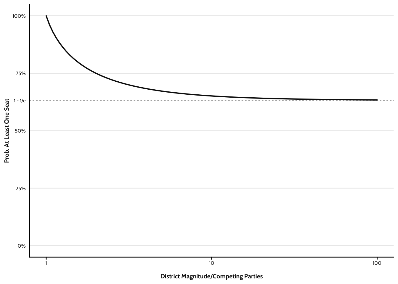
1. As we lack any data, we do not know each party’s popularity. So, our prior expectations must be flat: as far as we know, each party has exactly the same chance of winning any given seat. This then implies that the probability that any given party will win any given seat is $1/N_C^{\prime }$.

2. A nice trick when faced with a problem like this is to recognise that at least one success is the same as not all failures. Since we know that the probability of one success is $1/N_C^{\prime }$, we also know the probability of failure: $1-1/N_C^{\prime }$. And, as there are $M$ seats up for grabs, we must repeat this step $M$ times, giving ${(1-1/N_C^{\prime })}^M$.

3. Finally, since this equation tells us the probability of not winning a seat $M$ times in a row, we must convert it to successes. We can do this by subtracting it from 1, as follows: $1-{(1-1/N_C^{\prime })}^M$.

Thus, the probability that any given party will gain at least one seat, $Pr(m_i\ge 1)$, is:

$$Pr(m_i\ge 1)=1-{(1-\frac{1}{N_C^{\prime }})}^M$$

One nice thing about this equation is that as $M$ and $N_C^{\prime }$ tend to infinity, the probability that any given party will win at least one seat converges on $1-1/e\approx 0.63$. Figure 1 shows how quickly this occurs: with only 10 parties and 10 seats, convergence is almost total. So, all else being equal, any party that runs in a country like the Netherlands or Israel which has only a single nationwide district has around a 63% chance of winning at least one seat. Pretty good if you ask me!

Figure 1: All else being equal, the probability that any given party will win at least one seat in a district converges on around 63% as the number of parties and the district magnitude tend to infinity.

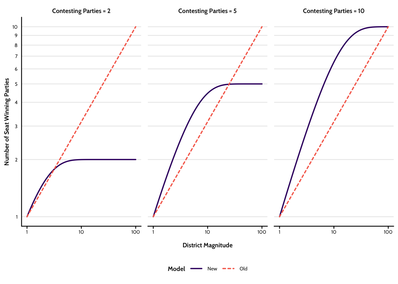
To complete the model, all we need to do is to multiply this probability by $N_C^{\prime }$, to give:

$$N_{S0}^{\prime }=N_C^{\prime }[1-{(1-\frac{1}{N_C^{\prime }})}^M]$$

Figure 2 plots predictions from this function as the district magnitude, $M$, increases from 1 to 100. Importantly, however, this simulation restricts the number of parties contesting the district, $N_C^{\prime }$, to 2, 5, and 10. As we can see, the old logical model continues to increase in line with $M$ even where it exceeds $N_C^{\prime }$. The newer model, however, does not and, instead, respects both possible ceilings.

Figure 2: Unlike the older logical model, one based on the occupancy problem does not allow for impossible values where the number of parties contesting some district is less than the district magnitude.

Final Steps

So far, the model makes predictions but lacks any parameters. This is a problem since we cannot either fit it to data or adjust the function’s slope. So we need some way to do this that still respect the known bounds that we set out above. The simplest way is to take $M$ to the power of some parameter, which we will call $\lambda$. This gives:

$$N_{S0}^{\prime }=N_C^{\prime }[1-{(1-\frac{1}{N_C^{\prime }})}^{M^{\lambda }}]$$

Figure 3: If we introduce a parameter to control the occupancy function’s slope, we know what bounds it must have. The smallest value it can take is 0, where one party wins all seats. The largest value it can take is 1, where a different party wins each seat.

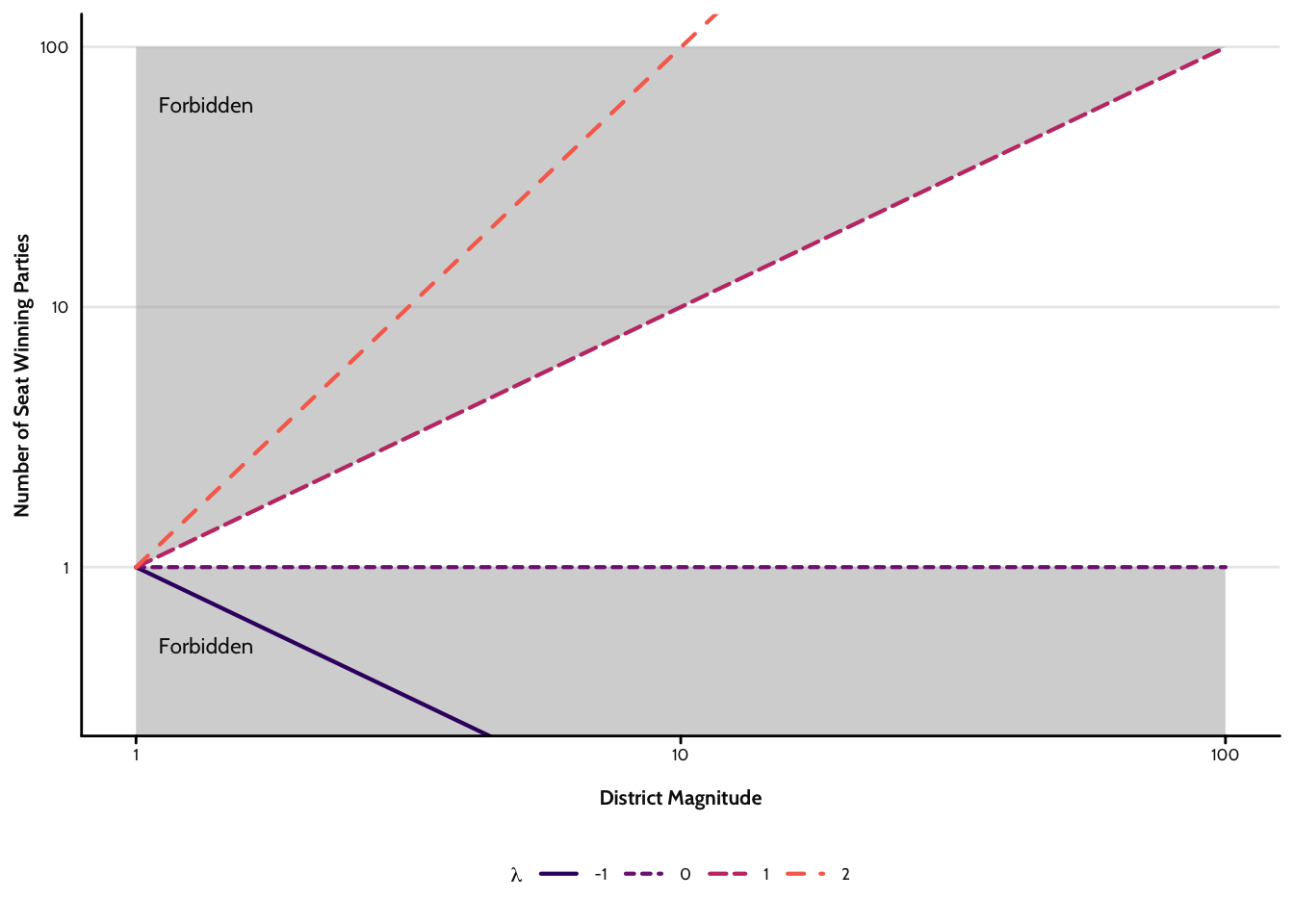
To complete our logical model, we need only determine the most likely value that $\lambda$ might take. Thankfully, this is not too hard. Figure 3 shows the model’s predictions after setting $N_C^{\prime }=10,000$ (to avoid any ceiling related to the number of competing parties) for four different values of $\lambda$: -1, 0, 1, and 2. I have also shaded two “forbidden areas” which logic dictates the slope must not enter. As we can see, the smallest value that $\lambda$ can take is 0. This corresponds to the case where one party wins all seats. Any lower than this, as $\lambda =-1$ shows, and the model would predict that the number of seat winning parties decreases as the district magnitudes grows. Obviously, this is impossible. Likewise, we can see that the largest value that $\lambda$ can take is 1, where a different party wins each seat. Higher than this, as $\lambda =2$ shows, and the model would predict more seat winning parties than seats: another logical impossibility.

Since we know $\lambda$’s bounds, our best guess at its value before we see any data is to take the mean of these two extremes, giving $\lambda =(0+1)/2=0.5$. This leads us to our final logical model:

$$N_{S0}^{\prime }=N_C^{\prime }[1-{(1-\frac{1}{N_C^{\prime }})}^{M^{1/2}}]$$

The really nice thing about this is that, in the limiting case where $N_C^{\prime }$ and $M$ tend to infinity, the function converges on the logical model that Shugart and Taagepera (2017) propose: $N_{S0}^{\prime }=M^{1/2}$. So their model is a limiting case of my model. Cumulative science in action! This model also results in a considerable bump in variation explained: an $R^2$ of 74% versus 65% for the older model. Obviously, $R^2$ isn’t the be all and end all: there are better ways to measure predictive accuracy. Still, since Shugart and Taagepera (2017) describe the model of district seat winning parties as a “fundamental building block” in all others that follow, improving our predictions here should feed forward into other models too. Regardless, it’s amazing how far we can get with only balls and urns!

References

Kollman, Ken, Allen Hicken, Daniele Caramani, David Backer, and David Lublin. 2024. “Constituency-Level Elections Archive.” Ann Arbor, MI.

McElreath, Richard. 2020. Statistical Rethinking: A Bayesian Course with Examples in R and Stan. 2nd ed. CRC Texts in Statistical Science. Boca Raton: CRC Press.

Shugart, Matthew S., and Rein Taagepera. 2017. Votes from Seats: Logical Models of Electoral Systems. Cambridge, UK: Cambridge University Press.

Taagepera, Rein. 2007. Predicting Party Sizes: The Logic of Simple Electoral Systems. Oxford: Oxford University Press.

———. 2008. Making Social Sciences More Scientific: The Need for Predictive Models. Oxford, UK: Oxford University Press.