In my last post, I discussed my remove some of the layers between the actual number of parties and derivatives like the effective number of parties and electoral disproportionality. That method focussed on building a logical model of the variance of party shares, breaking down the Gallagher index, and then using the former to model the latter. However, I was left stumped by a correlation coefficient and, after discussing the issue with Chris Hanretty, realised that that is where all the action is. As such, I’ve pivoted to another approach.
At the end of the post, I suggested some alternate ways forward. One was to develop a kind of “effective” measure of disproportionality that, much like the effective number of parties, is rooted in information theory. The general idea would be to measure disproportionality using the Rényi divergence. And, since we can decompose this measure into Rényi entropy and, therefore, into the effective number of parties, we might be able to get a better handle on the link between disproportionality and party-system fragmentation.
What follows is a preliminary attempt to elaborate such a measure along with some simple comparisons to the Gallagher index and a quick attempt at a constraint-based model.
Measuring Disproportionality
Political scientists most often measure disproportionality—the extent to which seat shares differ from vote shares—using the Gallagher index (Gallagher 1991).1 We compute the Gallagher index as follows:
Here,
“Effective” Disproportionality
If we were to begin the study of electoral systems again, we might seek to measure all electoral phenomena using some consistent framework. To this end, information theory would be a promising candidate. The reason it would be appealing is that the effective number of parties—perhaps the most important index in the study of elections—is information theoretic in nature. In particular, it shares an exact equivalence with the Rényi entropy, which is given as:
The parameter
Which is just the natural logarithm of the effective number of parties. So, by implication, those who have used the effective number of parties have worked with an information theoretic quantity for almost 50 years, whether they knew it or not.
Entropy measures, like the effective number of parties, measure how different some distribution is compared to uniformity. But this baseline is less useful if we want to measure disproportionality where we would instead prefer to compare one distribution to another. To do this, we can use the Rényi divergence, which compares two distributions and is given as follows:
Where
The logic here may not seem apparent at first, but consider that squaring any value and then dividing it by itself returns the original value. For instance,
Some Comparisons
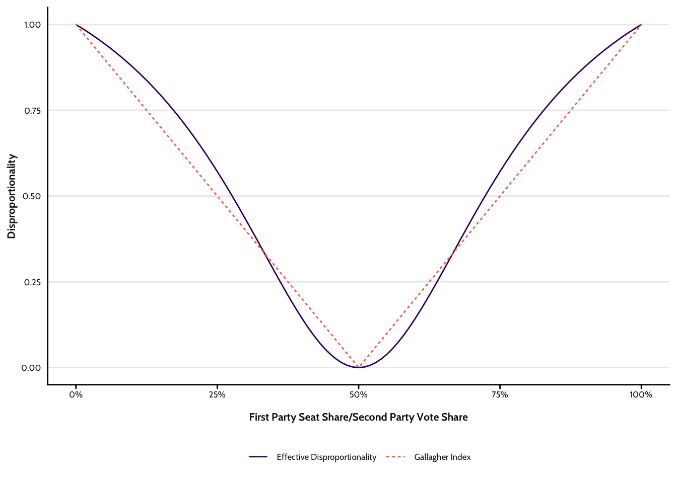
Figure 2 compare effective disproportionality to the Gallagher index using a simple simulated two party case. At the far left extreme of the horizontal axis, the first party has all of the votes and the second party all of the seats. At the half way point, both have an equal share of votes and seats. And, at the far right extreme, the picture flips. As we can see, both indices follow the same trajectory, though the effective measure curves whereas the Gallagher index does not. This, however, is specific to the two party case where the Gallagher index reverts to a simple measure of absolute difference (and outputs exactly the same values as the Pedersen index). In more complex scenarios where the number of parties is greater than two, the Gallagher index also curves.
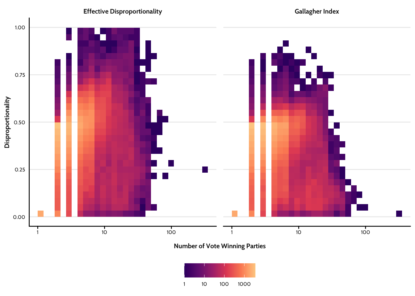
Figure 3 shows effective disproportionality (left panel) and the Gallagher index (right panel) plotted against the number of vote winning parties,
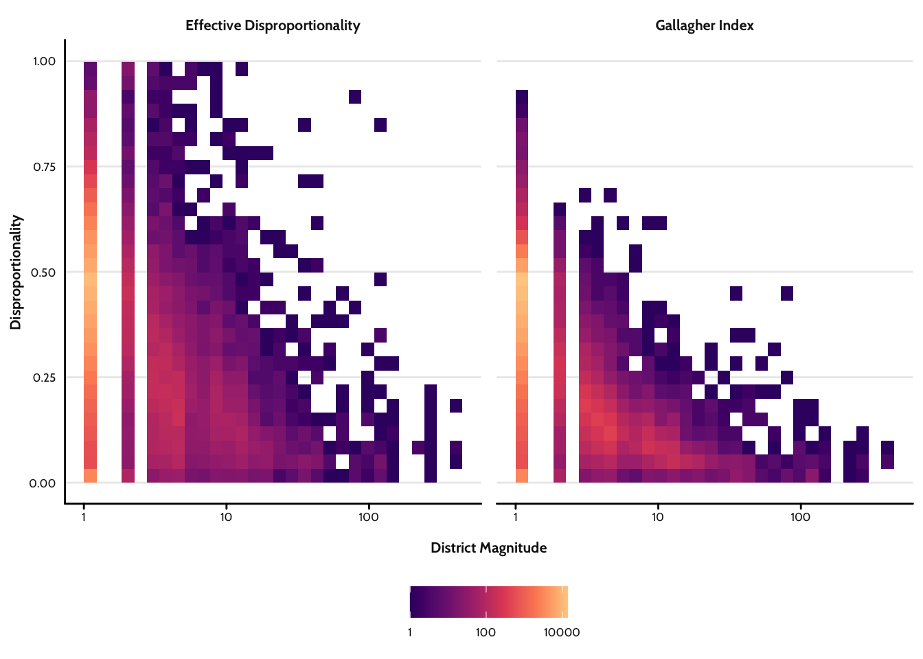
Figure 4 now shows effective disproportionality (left panel) and the Gallagher index (right panel) plotted against the district magnitude,
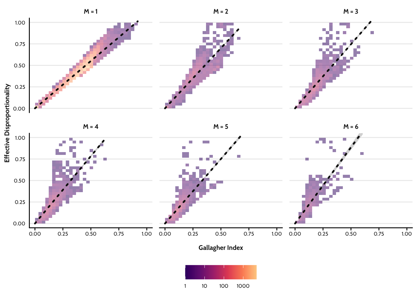
Finally, Figure 5 shows the two indices plotted against each other for districts with magnitudes of 1 to 6. In all cases, the two indices are highly correlated. Where
Steps Towards a Functional Form
So how might we build a logical model of effective disproportionality (or even disproportionality in general)? Absent any probabilistic logic that we might borrow, the most obvious way forward is to focus on constraints. As I mention above, one constraint is that where
What makes information theoretic quantities so useful is that they tend to have well known decompositions. One holds that
And since, as I show in this paper, the effective number of parties shares an exact equivalence with the Rényi entropy, such that
So, when the distribution of votes is perfectly uniform, disproportionality equals one minus the ratio of effective seat winning parties to actual vote winning parties. This feels like a nice property. I suspect we could also establish a similar constraint were we to focus on a uniform distribution of seats too. But, for now, I will stick to votes alone.
Though this model considers only a particular edge case, let’s see how well it does as a logical model of disproportionality. To test it, we’ll use it to predict disproportionality and then compare how much of the variation it explains in both effective disproportionality and the Gallagher index. We’ll also compare it to the current state of the art model that Shugart and Taagepera (2017) propose based on first estimating vote and seat shares for the first-placed party.
At the national level, the results are:
Existing method predicting the Gallagher index:
Existing method predicting effective disproportionality:
New model method predicting the Gallagher index:
New model predicting effective disproportionality:
And, at the district level (where
Existing method predicting the Gallagher index:
Existing method predicting effective disproportionality:
New model method predicting the Gallagher index:
New model predicting effective disproportionality:
In general, the model does well and more or less matches the current approach. Interestingly, however, the new model does well on both the effective disproportionality and the Gallagher index, whereas the current approach tends to do well for the Gallagher index but not the effective disproportionality. I’m going to wrap things up here, but I think this is a promising first step. Hopefully if we consider some further constraints, we might be able to improve it further still.
References
Footnotes
In Votes from Seats, Shugart and Taagepera (2017) refer to the index as
We sum over vote winning parties since not all vote winning parties are seat winning parties, but all seat winning parties are vote winning parties (at least in simple electoral systems).↩︎
Since seat shares may contain zeroes, we must use it as
This final step is only necessary when measuring disproportionality. To measure proportionality, subtracting from one is not necessary.↩︎
I use district level data here since they include more cases and include important edge cases where
At least in simple electoral systems.↩︎
Again, it must be the number of vote winning parties since we must sum over vote winning parties when computing the Rényi divergence.↩︎
